Le schéma de Lax-Wendroff

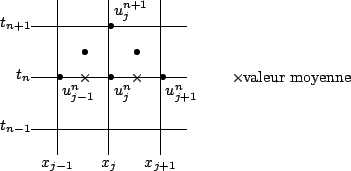
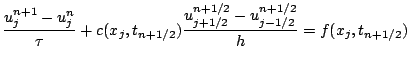
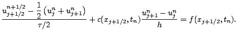
Des variables auxiliaires $u_{j + 1/2}^{n + 1/2}$ sont introduites aux points $x_{j + 1/2} = x_{j} + \dfrac{h}{2}$ et $t_{n + 1/2} = t_{n} + \dfrac{\tau}{2}$. Le schéma de Lax-Wendroff s'écrit :

$$\dfrac{u_{j}^{n+1} - u_{j}^{n}}{\tau} + c ( x_{j}, t_{n + 1/2} ) ... ...{u_{j + 1/2}^{n + 1/2} - u_{j - 1/2}^{n + 1/2}}{h} = f ( x_{j}, t_{n + 1/2} )$$

avec

$$\dfrac{u_{j + 1/2}^{n + 1/2} - \dfrac{1}{2} \left( u_{j}^{n} + u_... ... 1/2}, t_{n} ) \dfrac{u_{j+1}^{n} - u_{j}^{n}}{h} = f ( x_{j + 1/2}, t_{n} ).$$

Schématiquement, nous obtenons le diagramme suivant :

Nous verrons dans la suite que ce schéma est stable si $\tau\le h/\vert c_0\vert$.